transformer结束后开始学习图神经网络了。
看了GCN的论文,下面从使用与模型背后的数学原理分别介绍。
处理的数据集是Cora数据集,即半监督学习的分类问题,最后精度和论文差不多。
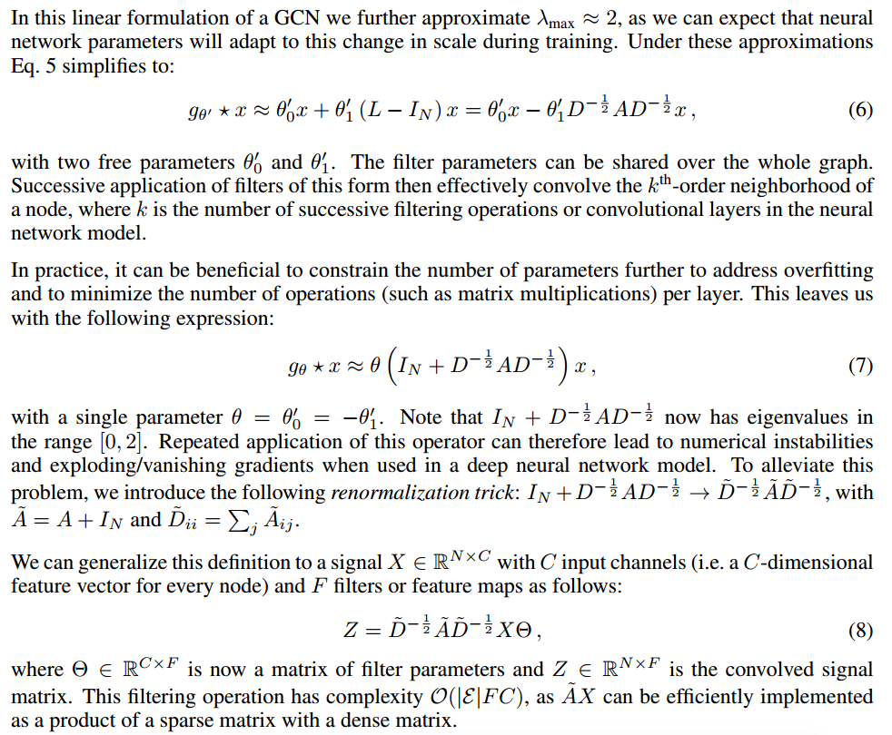
 # 直接使用 GCN的隐藏层传递公式如下:
其中DAD这一堆东西是可以从图的结构(即邻接矩阵)直接给出的。\(H^0=X,X=(x_1,x_2,...,x_c),x_i是图的第i个节点的特征向量。W=(w_1,...,w_f)是需要拟合的参数,f代表通道数(channels)(和CNN的通道数相似),w_i是一个过滤器(filter)\) 层传递公式就是这样,下面用pyg实现:

1
2
3
4
5
6
7
8
9
10
11
12
13
14
15
16
17
18
19
20
21
22
23
24
25
26
27
28
29
30
31
32
33
34
35
36
37
38
39
40
41
42
43
44
45
46
47
48
49
50
import torch
import torch.nn.functional as F
from torch_geometric import nn
from torch_geometric.data import Data
from torch_geometric.datasets import Planetoid

class GCN(torch.nn.Module):
def __init__(self, in_channels, hidden_channels, num_classify, dropout):
super().__init__()
self.conv1 = nn.GCNConv(in_channels, hidden_channels)
self.conv2 = nn.GCNConv(hidden_channels, num_classify)
self.dropout = torch.nn.Dropout(dropout)
def forward(self, graph):
x,edge_index = graph.x, graph.edge_index
h = F.relu(self.conv1(x,edge_index))
if self.training:
h = self.dropout(h)
o = self.conv2(h,edge_index)
return o

def test_accuracy(net, cora_data):
net.eval()
out = net(cora_data)
test_outs = out[cora_data.test_mask].argmax(dim=1)
test_labels = cora_data.y[cora_data.test_mask]
score = test_outs[test_outs==test_labels].shape[0]/test_outs.shape[0]
return score

dataset = Planetoid(root='./data/Cora', name='Cora')
cora_data = dataset[0]
hidden_channels = 32
epochs, lr = 200, 0.01
weight_decay = 5e-4

net = GCN(cora_data.num_features, hidden_channels, dataset.num_classes, 0.2)
optimizer = torch.optim.Adam(net.parameters(), lr=lr, weight_decay=weight_decay)
loss_fn = torch.nn.CrossEntropyLoss()

device = torch.device('cuda')
net = net.to(device)
cora_data = cora_data.to(device)
for e in range(epochs):
y_hat = net(cora_data)
optimizer.zero_grad()
loss = loss_fn(y_hat[cora_data.train_mask], cora_data.y[cora_data.train_mask])
loss.backward()
optimizer.step()

print(f'epoch:{e}, loss:{loss.item()}')
print(test_accuracy(net, cora_data))
最后输入测试集准确率为0.812

从零实现GCN网络

1
2
3
4
5
6
7
8
9
10
11
12
13
14
15
16
17
18
19
20
21
22
23
24
25
26
27
28
29
30
31
32
33
34
35
36
37
38
39
40
41
42
43
44
45
46
47
48
49
50
51
52
53
54
55
56
57
58
59
60
61
62
63
64
65
66
67
68
69
70
71
72
73
74
75
76
77
78
79
80
81
82
83
84
85
86
87
88
89
90
91
92
93
94
95
96
97
98
99
100
import torch
from torch import nn
import torch.nn.functional as F
from scipy.sparse import csr_matrix, coo_matrix
import scipy.sparse as sp
import numpy as np
import matplotlib.pyplot as plt

adj_path = 'Graph/data/Cora/cora.cites'
node_path = 'Graph/data/Cora/cora.content'

def sparse_mx_to_torch_sparse_tensor(sparse_mx):
"""Convert a scipy sparse matrix to a torch sparse tensor."""
sparse_mx = sparse_mx.tocoo().astype(np.float32)
indices = torch.from_numpy(
np.vstack((sparse_mx.row, sparse_mx.col)).astype(np.int64))
values = torch.from_numpy(sparse_mx.data)
shape = torch.Size(sparse_mx.shape)
return torch.sparse_coo_tensor(indices, values, shape)

def load_cora(adj_path, node_path):
nodes = np.genfromtxt(node_path, dtype=str)
# 节点特征向量
features = csr_matrix(nodes[:,1:-1], dtype=np.float64)
# 节点编号
idx = np.array(nodes[:,0], dtype=np.int32)
idx_map = {j:i for i,j in enumerate(idx)}
# 标签
labels = nodes[:,-1]
classes = set(list(labels))
classes_map = {c:i for i,c in enumerate(classes)}
labels = np.array(list(map(classes_map.get, labels)))

edges = np.genfromtxt(adj_path, dtype=np.int32)
# 将论文索引与顶点编号对应,然后使用稀疏矩阵
adj = np.array(list(map(idx_map.get, edges.flatten()))).reshape(edges.shape)
# 此时构造的矩阵是一个上三角矩阵,因为论文编号小的论文是不会引用比它编号大的论文
coo_adj = coo_matrix((np.ones(adj.shape[0]), (adj[:,0], adj[:,1])),
shape=(idx.shape[0], idx.shape[0]), dtype=np.int32)
coo_adj = coo_adj+coo_adj.T+sp.eye(coo_adj.shape[0])
d = np.array(coo_adj.sum(1))
d = sp.diags(np.power(d, -1/2).flatten())
adj_hat = d@coo_adj@d

# to tensor
adj_hat = sparse_mx_to_torch_sparse_tensor(adj_hat)
features = sparse_mx_to_torch_sparse_tensor(features)
labels = torch.LongTensor(labels)

return adj_hat, features, labels, idx_map, classes_map

class GCN(nn.Module):
def __init__(self, in_channels, hidden_channels, num_classify, dropout, bias=False):
super().__init__()
self.conv1 = nn.Linear(in_channels, hidden_channels, bias=bias)
self.conv2 = nn.Linear(hidden_channels, num_classify, bias=bias)
self.dropout = nn.Dropout(dropout)
def forward(self, x, adj):
h = F.relu(adj@self.conv1(x))
if self.training:
h = self.dropout(h)
o = adj@self.conv2(h)
return o

def test_accuracy(net, x, adj, y):
net.eval()
out = net(x, adj)
test_outs = out[140:1140].argmax(dim=1)
score = test_outs[test_outs==y].shape[0]/test_outs.shape[0]
return score


adj, X, Y, idx_map, classes_map = load_cora(adj_path, node_path)
hidden_channels = 32
epochs, lr = 200, 0.01
weight_decay = 5e-4

net = GCN(X.shape[1], hidden_channels, len(classes_map), 0.2)
optimizer = torch.optim.Adam(net.parameters(), lr=lr, weight_decay=weight_decay)
loss_fn = torch.nn.CrossEntropyLoss()

device = torch.device('cuda')
net = net.to(device)
adj, X, Y = [e.to(device) for e in [adj, X, Y]]

if __name__=='__main__':
loss_list = []
for e in range(epochs):
y_hat = net(X, adj)
optimizer.zero_grad()
loss = loss_fn(y_hat[range(140)], Y[range(140)])
loss.backward()
optimizer.step()

loss_list.append(loss.item())
if e%10==0:
print(f'epoch:{e}, loss:{loss.item()}')
print(test_accuracy(net, X, adj, Y[140:1140]))
plt.plot(loss_list)
plt.show()

输出精度为0.832

数学原理

参考链接

数学分析之投影内积和傅里叶级数
GCN原理(写的很好!)
Graph Neural Network (2/2) (由助教姜成翰同學講授)
【双语字幕】斯坦福CS224W《图机器学习》课程(2021) by Jure Leskovec
「珂学原理」No. 26「拉普拉斯变换了什么?」
纯干货数学推导_傅里叶级数与傅里叶变换
B站首发!草履虫都能看懂的【傅里叶变换】讲解,清华大学李永乐老师教你如何理解... ## 个人理解 pass

原文的一些备注

  • diag(x),x is vector.将向量x对角化。

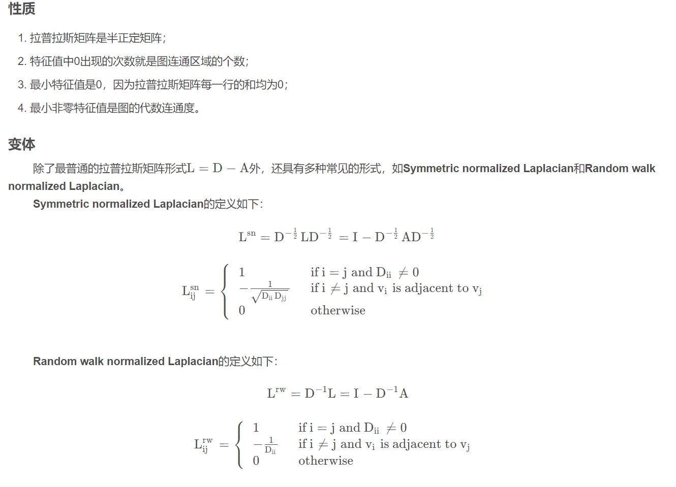
  • sys normalized laplacian matrix
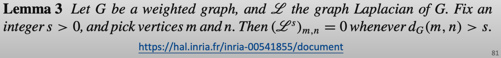
image-20240310180048878
  • 图论的一个定理image-20240310181611507

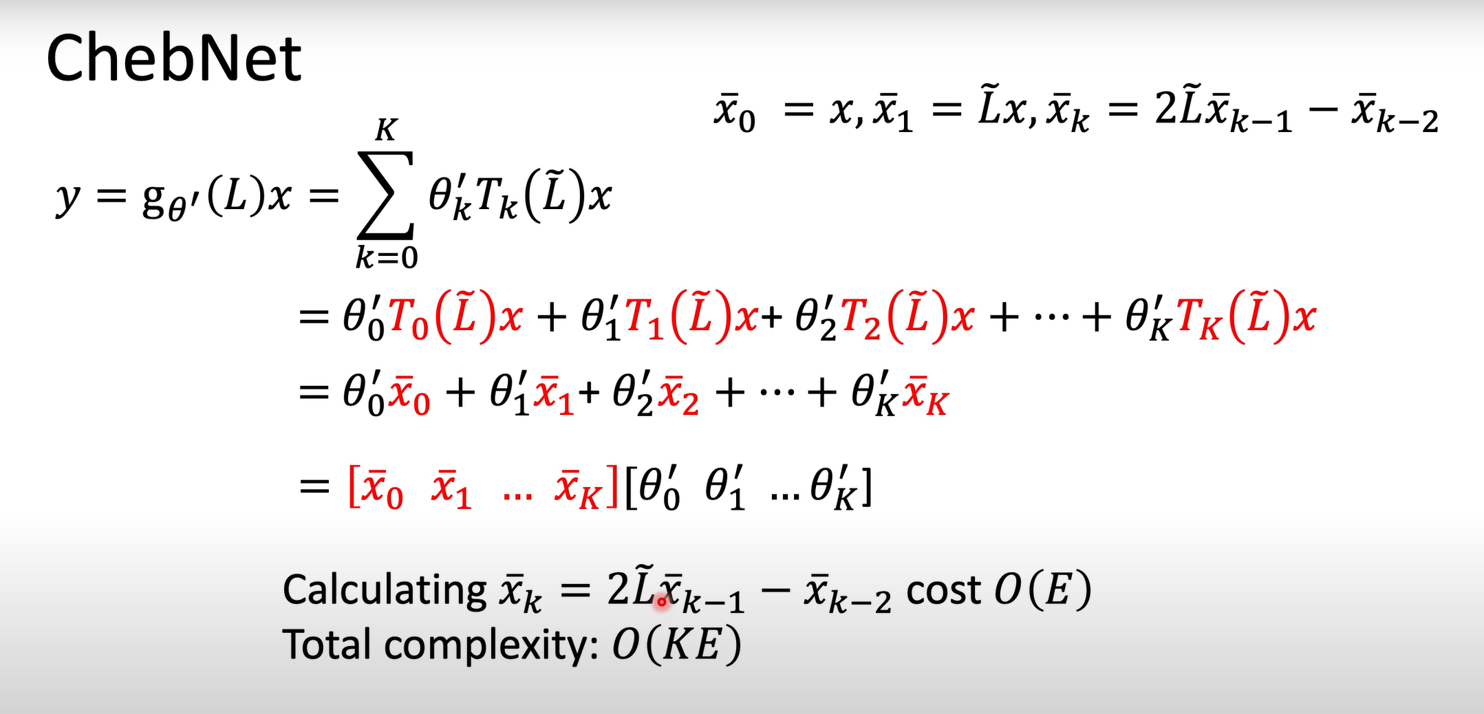
  • Chebyshev Polynomial(切比雪夫多项式)image-20240310184134296

    wiki

  • GCN对Fourier domain的变体image-20240310194416895