1
2
3
4
5
6
7
8
9
10
11
12
13
14
15
16
17
18
19
20
21
22
23
24
25
26
27
28
29
30
31
32
33
34
35
36
37
38
39
40
41
42
43
44
45
46
47
48
49
50
51
52
53
54
55
56
57
58
59
60
61
62
63
64
65
66
67
68
69
70
71
72
73
74
75
76
77
78
79
80
81
82
83
84
85
86
87
88
89
90
91
92
93
94
95
96
97
98
99
| import torch
import torchvision
from torchvision import transforms
from torch.utils import data
import matplotlib.pyplot as plt
from torch import nn
mnist_train = torchvision.datasets.FashionMNIST(
root='../data', train=True, transform=transforms.ToTensor(), download=True
)
mnist_test = torchvision.datasets.FashionMNIST(
root='../data', train=False, transform=transforms.ToTensor(), download=True
)
def softmax(x):
x_exp = torch.exp(x)
return x_exp/x_exp.sum(1, keepdim=True)
def net(x, w1, b1, w2, b2):
h = torch.matmul(x.reshape((-1, w1.shape[0])), w1)+b1
y = torch.matmul(torch.relu(h), w2)+b2
return softmax(y)
def cross_entropy(y, y_hat):
return - torch.log(y_hat[range(len(y_hat)), y])
def sgd(params, lr, batch_size):
with torch.no_grad():
for param in params:
param -= lr*param.grad/batch_size
param.grad.zero_()
def ac(w1, b1, w2, b2, data_iter, net):
num_acs = []
for x, y in data_iter:
y_hat = net(x, w1, b1, w2, b2)
maxs, indexs = torch.max(y_hat, dim=1)
num_acs.append(y.eq(indexs).sum()/indexs.shape[0])
return sum(num_acs)/len(num_acs)
batch_size = 256
train_iter = data.DataLoader(
mnist_train, batch_size, shuffle=True, num_workers=4)
test_iter = data.DataLoader(mnist_test, batch_size,
shuffle=True, num_workers=4)
lr = 0.1
num_epochs = 10
net = net
loss = cross_entropy
num_output = 10
num_input = 28*28
num_hidden = 256
w1 = torch.normal(0, 0.1, (num_input, num_hidden), requires_grad=True)
b1 = torch.zeros(num_hidden, requires_grad=True)
w2 = torch.normal(0, 0.1, (num_hidden, num_output), requires_grad=True)
b2 = torch.zeros(num_output, requires_grad=True)
if __name__ == '__main__':
train_acs = []
test_acs = []
losss = []
for i in range(num_epochs):
for x, y in train_iter:
y_hat = net(x, w1, b1, w2, b2)
l = loss(y, y_hat)
l.sum().backward()
sgd([w1, b1, w2, b2], lr, batch_size)
train_ac = ac(w1, b1, w2, b2, train_iter, net)
test_ac = ac(w1, b1, w2, b2, test_iter, net)
train_acs.append(train_ac)
test_acs.append(test_ac)
losss.append(l.sum().detach().numpy())
print('epoch:{}, train iter ac:{}, test iter ac:{}'.format(
i, train_ac, test_ac))
fig, axes = plt.subplots(1,2, figsize=(8,2))
axes = axes.flatten()
axes[0].plot(range(10), losss)
axes[1].plot(range(10), train_acs, label='train data')
axes[1].plot(range(10), test_acs, label='test data')
axes[1].legend()
|
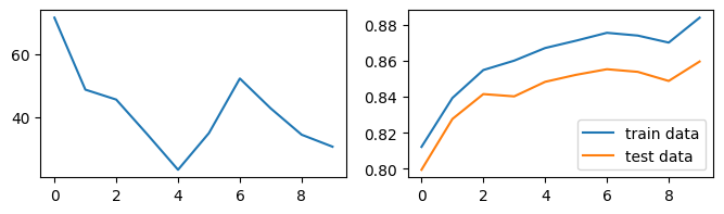 发现准确率也不够高!