函数原型

\[ h_\theta(X)=\frac{1}{1+e^{-\theta^TX}}...称h_\theta(X)为y=1的概率。 \]

决策界限的定义

根据函数表达式可知当$z>=0$时$y>=0.5$当$z<0$时$y<0.5...z=\theta^TX,y=h_\theta(X)$

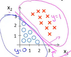
$故直线z=\theta^TX为决策界限$

代价函数

线性回归的代价函数为：

\[ J(\theta)=2\frac{1}{m}\sum_{i=1}^{m}(h_\theta(x^i)-y(x^i))^2 \]

我们另：

\[ J(\theta)=\frac{1}{m}\sum_{i=1}^{m}Cost(h_\theta(x^i),y(x^i)) \]

$Cost为：$

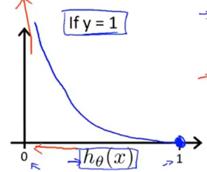
\[ Cost(h_\theta(x^i),y(x^i))=\begin{cases} -log(h_\theta (x))& \text if&y=1\\-log(1-h_\theta (x))& \text if&y=0\end{cases} \]

为什么这样选择？

$-log(1-h_\theta (x))图像为：$

其中

\[ h_\theta(X)=\frac{1}{1+e^{-\theta^TX}}. \]

当$h_\theta (x)$无限靠近与0时，代价函数为无穷大。故$h_\theta (x)=0$表示y=1的概率为0，与条件y=1完全矛盾。故给该算法加大惩罚。$

当$h_\theta (x)$无限靠近与1时，代价函数为0。故$h_\theta (x)=1$表示y=1的概率为100%，与条件y=1完全符合。

$-log(1-h_\theta (x))图像为：$

证明方式与图1类似...

合并代价函数

\[ J(\theta)=\frac{1}{m}\sum_{i=1}^m(-ylog(h_{\theta}(x^i))-(1-y)log(1-h_{\theta}(x^i))) \]

使用梯度下降法迭代

公式与线性回归公式相同。证明参考：https://blog.csdn.net/qq_29663489/article/details/87276708 ## 多分类问题

思想：二分，归类于y=1概率的的一类。如图，三个函数同时处理，得到$h_\theta(X)$，故点归类于$h_\theta(X)$大的一类。

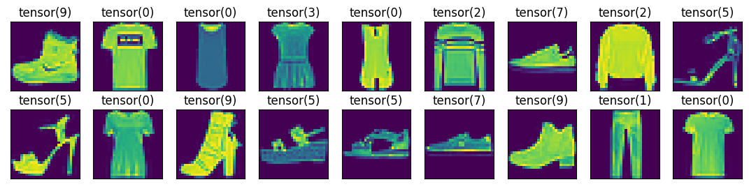
d2l 从零实现

读取mnist数据集

import torch
import torchvision
from torchvision import transforms
from torch.utils import data
import matplotlib.pyplot as plt

mnist_train = torchvision.datasets.FashionMNIST(
    root='../data', train=True, transform=transforms.ToTensor(), download=True
)
mnist_test = torchvision.datasets.FashionMNIST(
    root='../data', train=False, transform=transforms.ToTensor(), download=True
)

def show_images(imgs, num_rows, num_cols, titles=None, scale=1.5):
    figsize = (num_cols*scale, num_rows*scale)
    _, axes = plt.subplots(num_rows, num_cols, figsize=figsize)
    axes = axes.flatten()
    for i, (ax,img) in enumerate(zip(axes, imgs)):
        ax.imshow(img.numpy())
        ax.set_title(titles[i])
        ax.axes.get_xaxis().set_visible(False)
        ax.axes.get_yaxis().set_visible(False)
    return axes

batch_size = 18
x,y = next(iter(data.DataLoader(mnist_train, batch_size=batch_size)))
show_images(x.reshape(batch_size, 28, 28), 2, 9, titles=y)

train

# 前向传播
def softmax(x):
    x_exp = torch.exp(x)
    return x_exp/x_exp.sum(1, keepdim=True)

def net(x, w, b):
    # x shape (batch_size, 28*28)
    # w (28*28, 10)
    y = torch.matmul(x.reshape((-1, w.shape[0])),w)+b
    return softmax(y)

# 代价函数
def cross_entropy(y, y_hat):
    return  - torch.log(y_hat[range(len(y_hat)), y])

# sgd
def sgd(params, lr, batch_size):
    with torch.no_grad():
        for param in params:
            param -= lr*param.grad/batch_size
            param.grad.zero_()

# y = torch.tensor([0])
# y_hat = torch.tensor([[0.6, 0.3, 0.1]])
# cross_entropy(y, y_hat)

# 准确率
def ac(w, b, data_iter, net):
    for x,y in data_iter:
        y_hat = net(x,w,b)
        maxs, indexs = torch.max(y_hat, dim=1)
        num_ac = y.eq(indexs).sum()/indexs.shape[0]
        return num_ac

# 准备数据
batch_size = 256
train_iter = data.DataLoader(mnist_train, batch_size, shuffle=True, num_workers=4)
test_iter = data.DataLoader(mnist_test, batch_size, shuffle=True, num_workers=4)

# 超参数
lr = 0.1
num_epochs = 10
net = net
loss = cross_entropy

# 参数
num_out = 10
num_input = 28*28
w = torch.normal(0, 0.01, (28*28, 10), requires_grad=True)
b = torch.zeros(num_out, requires_grad=True)

# 训练
for i in range(num_epochs):
    for x,y in train_iter:
        y_hat = net(x, w, b)
        l = loss(y, y_hat)
        l.sum().backward()
        sgd([w,b], lr, batch_size)
    print('epoch:{}, ac:{}'.format(i, ac(w, b, train_iter, net)))

# epoch:0, ac:0.82421875
# epoch:1, ac:0.81640625
# epoch:2, ac:0.828125
# epoch:3, ac:0.81640625
# epoch:4, ac:0.875
# epoch:5, ac:0.8359375
# epoch:6, ac:0.8515625
# epoch:7, ac:0.85546875
# epoch:8, ac:0.8515625
# epoch:9, ac:0.8984375

保存参数

torch.save(w, 'w.pt')
torch.save(b, 'b.pt')

w = torch.load('w.pt')
b = torch.load('b.pt')

d2l 简洁实现

nn.Flatten与torch.flatten的区别

a = torch.arange(24).reshape((2,3,4))
f = nn.Flatten()
# nn.Flatten()的第一个维度一般是batch
f(a).shape, torch.flatten(a).shape

# (torch.Size([2, 12]), torch.Size([24]))

实现

def ac(data_iter, net):
    for x,y in data_iter:
        y_hat = net(x)
        maxs, indexs = torch.max(y_hat, dim=1)
        num_ac = y.eq(indexs).sum()/indexs.shape[0]
        return num_ac

def init_weights(m):
    if type(m) == nn.Linear:
        nn.init.normal_(m.weight, std=0.01)

net = nn.Sequential(nn.Flatten(), nn.Linear(28*28, 10))
net.apply(init_weights)
loss = nn.CrossEntropyLoss(reduction='none')
trainer = torch.optim.SGD(net.parameters(), lr=lr)

for i in range(num_epochs):
    for x,y in train_iter:
        y_hat = net(x)
        l = loss(y_hat, y)
        trainer.zero_grad()
        l.sum().backward()
        trainer.step()
    print('epoch:{}, ac:{}'.format(i, ac(train_iter, net)))

# epoch:0, ac:0.7421875
# epoch:1, ac:0.78515625
# epoch:2, ac:0.7890625
# epoch:3, ac:0.82421875
# epoch:4, ac:0.81640625
# epoch:5, ac:0.8125
# epoch:6, ac:0.84375
# epoch:7, ac:0.8515625
# epoch:8, ac:0.82421875
# epoch:9, ac:0.8125

QA

net = nn.Sequential(nn.Flatten(), nn.Linear(28*28, 10))为什么没有Softmax层？

nn.CrossEntropyLoss(reduction='none')？
softmax层在CrossEntropyLoss中：nn.CrossEntropyLoss

loss_func = nn.CrossEntropyLoss()
pre = torch.tensor([[0.8, 0.5, 0.2, 0.5]], dtype=torch.float)
tgt = torch.tensor([[1, 0, 0, 0]], dtype=torch.float)

cross_entropy(0, torch.softmax(pre, dim=1)), loss_func(pre, tgt)

# (tensor([1.1087]), tensor(1.1087))

机器学习学习的Logistic回归算法